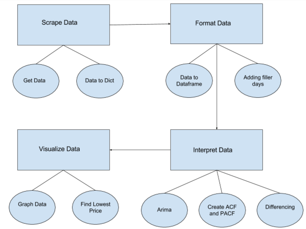
In order to make our code more manageable, we divided it into four classes: Collecter, Formatter, Interpreter, and Visualizer. As these names indicate, the Collecter class grabs the data from a source online and the Formatter class arranges the data into a dataframe that is then passed into the Interpreter class. The Interpreter then uses the data frame and passes it into the model, which predicts price values. These values are passed to the Visualizer which creates images of the predicted prices and past prices. When the user interacts with our web application, they choose a product and our application predicts the future price of that product at the specified time frame.
The following model demonstrates the layout of our web application.
 The Seasonal Auto Regression Integrated Moving Average (SARIMA) model functions by finding the future prices based on the previous prices. Since product prices vary with season - for example, electricity prices change in respect to seasons - the model requires parameters for the seasonality and stationarity of our data. In order to account for this seasonality we decomposed the data using seasonal decomposition. Since SARIMA needs time series to be stationary, meaning that they were independent of time, we took the difference between the prices and their previous values. We also made the seasonality trend stationary by differencing it.
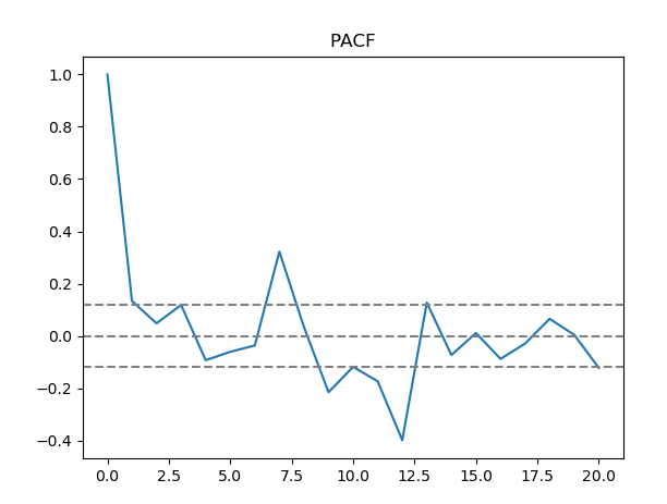
Once we had our stationary data and seasonality data, we found the parameters that would go into the model. We needed to determine the number of autoregression terms and lagged forecast errors for both the stationarity and seasonality data. One way to find the number of autoregression terms was by calculating, to the nearest integer, the first moment of the second standard deviation of the autocorrelation function for both the stationarity and seasonality data. In order to determine the lagged forecast errors we found the first time the second standard deviation of the partial autocorrelation function was reached. After calculating these values, we now had all the p and q parameters for our model.
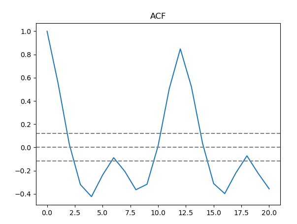
Autocorrelation function of differenced prices.
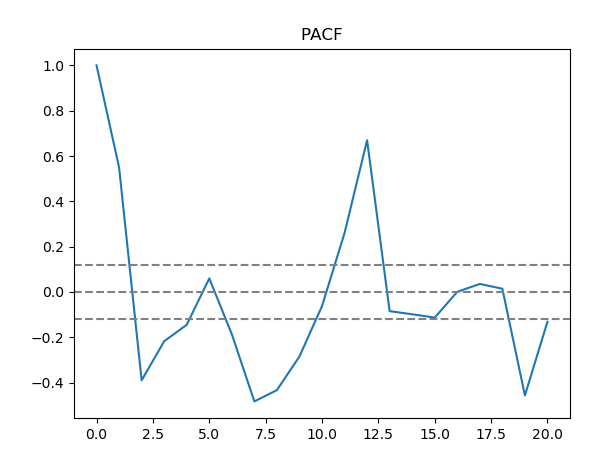
Partial autocorrelation function of differenced prices.
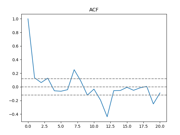
Autocorrelation function of seasonality in prices.
Partial autocorrelation function of seasonality in prices.
The Interpreter class then passes the data and its parameters into a SARIMA model which determines the prediction values for the requested number of days. This data is then passed into a Visualizer object which graphs the data, while also returning what day will have the lowest price. The script for our website then calls this function, in order to output the lowest price and the graph to the user.